THERMOCOUPLES AND THERMOCOUPLE SLIP RING CIRCUITS
A simple thermocouple circuit is shown in Figure 1.
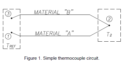
Let points 1 and 3 be thermally integrated i.e. the temperature at point 1 always equals the temperature at point 3 and let this temperature equal Tref. If the temperature at point 2 does not equal the reference temperature (T2 ≠ Tref), there is an end-to-end voltage or electromotive force (EMF) generated along the length of material “A” wire and another endto-end EMF generated along the length of material “B” wire. The magnitude of the EMF generated along a particular wire is a function of the temperature difference or integrated gradient along the wire. By algebraically summing voltages, the EMF between 1 and 3 is equal to the EMF from 1 to 2 plus the EMF from 2 to 3. Therefore the magnitude of the EMF developed between points 1 and 3 is a function of the temperature at point 2. Hence, the connection or junction of the two thermocouple wires at point 2 defines the location of where temperature is sensed as well as serving to complete the electrical circuit – EMF is not generated at junction point 2.
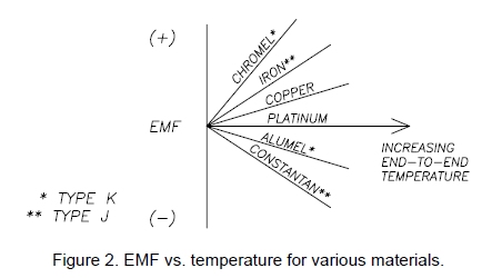
Figure 2 shows the EMF versus temperature behavior of several common thermocouple materials referred to platinum. Note that the two materials used to make a thermocouple type (e.g. K-type, J-type, etc.) are those that exhibit a “large” mutual divergence.
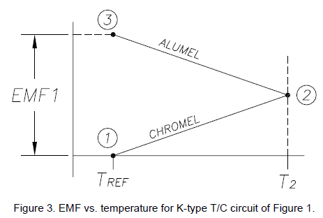
The EMF versus temperature plot of the circuit depicted in Figure 1 for a K-type thermocouple is shown in Figure 3.
Refer back to Figure 1. Since the EMF’s generated are dependent upon the differences of temperature, we need to know the temperature of points 1 and 3 in order to measure the temperature at point 2. Furthermore, we need a means of connecting points 1 and 3 to a readout device (e.g. a voltmeter) and the leadwires to this device will introduce another material (e.g. copper) that is subject to thermal EMF generation.
Figure 4 shows the circuit of Figure 1 using K-type thermocouple materials and now includes a readout device with leadwires and a reference temperature zone held at Tref. The EMF versus temperature plot for this arrangement is shown in figure 5.
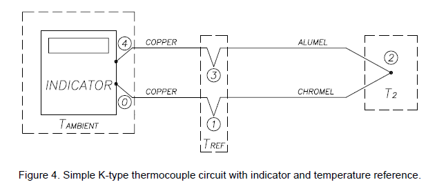
Examination of figure 5 reveals that the introduction of the copper leadwires has no effect upon the output EMF as long as points 0 and 4 are at the same temperature.
We still however need a means of holding both points 1 and 3 at some known temperature, Tref. Historically, this has been achieved through the use of an ice bath. (Consequently, published thermocouple tables usually provide output voltage with respect to a reference junction temperature of 0° C or 32° F.)
Since ice baths are not usually practical to implement, other methods to obtain or emulate a reference junction have been developed. One method utilizes an electrical resistance bridge circuit that contains a temperature sensitive resistor element. The bridge circuit is placed in series with the thermocouple circuit and is thermally integrated with the reference junction points 1 and 3. With points 1 and 3 at 0° C, the bridge does not introduce any voltage. However, when points 1 and 3 deviate from 0° C, say for example to the ambient temperature of the indicator, the bridge will introduce a voltage equal and opposite to the voltage change at the reference junction thus maintaining an equivalent 0° C reference junction temperature.
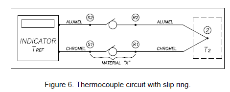
CONSEQUENCE OF INTRODUCING A SLIP RING (OR CONNECTOR) BETWEEN THE INDICATOR AND THE MEASUREMENT POINT.
Figure 6 shows the circuit of Figure 4 with a slip ring placed between the indicator and measurement point 2, where S1 and S2 are slip ring stator terminals and R1 and R2 are the corresponding slip ring rotor terminals respectively. Note that the reference junction discussed above is physically located within the “INDICATOR”.
If there is no temperature difference between the stator and the rotor terminals, the temperature at S1 equals the temperature at R1 and the temperature at S2 equals the temperature at R2. The EMF vs. temperature graph for this case is shown in Figure 7.
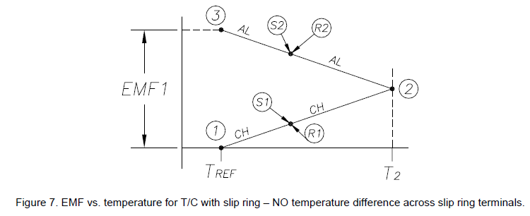
Since there is no temperature difference, ΔT=0 across the slip ring material and the stator and rotor connection points overlay each other on the graph. In this case there will be no error in measurement. However, if a temperature difference does exist across the slip ring, the EMF versus temperature graph will look like that shown in Figure 8.
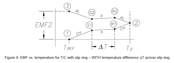
In this case EMF2 < EMF1 and the measurement is in error. Examination of this plot shows that the actual temperature of the test part at point 2 is higher than would be indicated by an amount equal to ΔT.
In the previous example the temperature of the rotor was taken to be greater than the stator. If the stator temperature is greater than the rotor temperature the EMF vs. temperature diagram will look as shown in Figure 9.
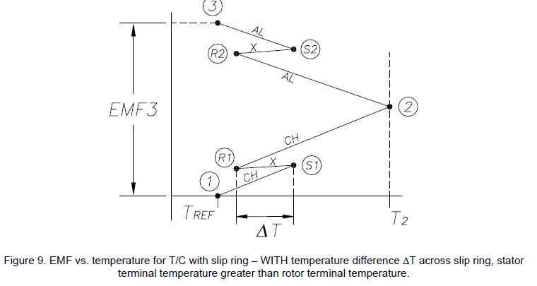
Note that EMF3 > EMF1. The actual temperature of the test part at point 2 is lower than would be indicated by an amount equal to ΔT. This discussion has been simplified in that actual slip ring assemblies can contain several connections of various materials between the stator and rotor terminals proper. Each of these connections are in turn subject to the kind of temperature gradient errors discussed and will combine with the error associated with the stator and rotor terminal connections to produce a net error.
Temperature gradient errors associated with slip rings can be eliminated by placing a thermocouple amplifier (with built-in “cold junction” reference) on the spinning side of the slip ring as shown in Figure 10. Compare this figure to Figure 6. In this arrangement the slip ring is no longer in series with the thermocouple wire and therefore temperature differences across the slip ring will not manifest themselves as measurement error.
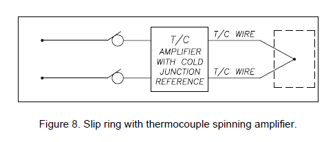
Michigan Scientific makes Spinning Thermocouple Amplifiers for end of shaft and tubular type slip rings. These amplifiers contain a cold junction reference and provide gain to improve the signal to noise ratio.
The temperature gradient and graphical analysis approach used to describe thermocouple behavior in this tech note is patterned after that presented by Dr. Robert J. Moffat in an article reprinted in Applied Measurement Engineering by Charles P. Wright, Prentice Hall, 1995. This article is suggested reading for further information about thermocouple theory and practice.